Tutorial 1: Denoising on single-slice DLPFC data from 10x Visium

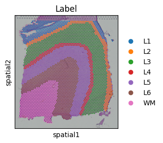
In this tutorial, we demonstrate the denoising capabilities of STADIM using single-slice data. We use the human Dorsolateral Prefrontal Cortex (DLPFC) slice #151673 generated by 10x Visium platform as a representative example, which is annotated by Maynard et al. into white matter (WM) and cortical layers (L1-L6) based on marker genes and cellular structure.

We download the data via http://spatial.libd.org/spatialLIBD/.

Quick view data

[1]:

import anndata as ad

raw_data = ad.read_h5ad('/data2/xiaost/SODA/Data/DLPFC/dlpfc_151673.h5ad')

print(raw_data)

AnnData object with n_obs × n_vars = 3611 × 33538
    obs: 'in_tissue', 'array_row', 'array_col', 'sample', 'Label'
    var: 'gene_ids', 'feature_types', 'genome'
    uns: 'spatial'
    obsm: 'spatial'

[2]:

print(raw_data.obs.head(5))

                    in_tissue  array_row  array_col  sample Label
AACGTGATGAAGGACA-1          1          9         83  151673    L3
TGATTCCCGGTTACCT-1          1         64         50  151673    L6
CTTTGGCGCTTTATAC-1          1         32         18  151673    L4
ACGCTGTGAGGCGTAG-1          1         39         13  151673    L5
AGGTTACACCATGCCG-1          1         43        115  151673    L2

[3]:

import scanpy as sc
import matplotlib.pyplot as plt

fig, ax = plt.subplots(figsize=(3, 3))
sc.pl.spatial(raw_data, color='Label', ax=ax, show=False)
plt.show()

Run STADIM

You can call the STADIM command directly in your terminal:

nohup stadim --input "./dlpfc_151673.h5ad" --save_dir ./dlpfc_151673_test --device "cuda:0" --monitor --seed 2026 --min_genes 0 --min_cells 10 --knn_c 6 --knn_e 10 > ./dlpfc_151673_test.log 2>&1 &

and load the results into your Python environment for downstream analysis. The denoised expression matrix is conveniently stored within the layers attribute:

import anndata as ad

adata = ad.read_h5ad('/dlpfc_151673_test/sdata.h5ad')

## The denoised gene expressionis is stored in adata.layers['STADIM']
print(adata)

or you can call STADIM within a Jupyter Notebook as follows:

[4]:

import stadim

adata = stadim.run_STADIM(['/data2/xiaost/SODA/Data/DLPFC/dlpfc_151673.h5ad'], save_preprocessed_h5ad=None, save_dir=None,
                          sample_names=None, batch_key='sample', device='cuda:1', seed=2026,
                          min_genes=0, min_cells=10, nhvgs=2000, dim=50, knn_c=6, knn_e=10, mnn_n=25,
                          batch_size=256, triplets_update_ratio=0.8, hard_triplets_ratio=0.7,
                          epochs=100, lr=1e-3, loss_mode='nb', beta_trip=0.1,
                          encoder_layers=[512, 256, 64], decoder_layers=[1000])

Results will be stored in adata.layers['STADIM']

=== 1. Begin read_data!
Processing single slice: Using user-defined column 'sample'
Processing single slice: Keeping existing sample label 151673

Merging data...

Raw Merged Data: 3611 spots × 33538 genes
Unified Filtering (min_genes=0, min_cells=10)...
  → After Filtering: 3611 spots × 16567 genes
  ✓ Complete: Samples included: ['151673']
  ✓ Complete: AnnData object with n_obs × n_vars = 3611 × 16567
    obs: 'in_tissue', 'array_row', 'array_col', 'sample', 'Label'
    var: 'gene_ids', 'feature_types', 'genome', 'n_cells'
    uns: 'spatial'
    obsm: 'spatial'
    layers: 'X_raw'

=== 2. Begin MY_preprocess!
== Selected 2000 HVGs across 1 slices

=== 3. Begin all_ap find neighbors!

=== 4. Begin pre_dataset!
{0: '151673'}

Preparing triplet: 100%|██████████| 3611/3611 [00:00<00:00, 6602.14it/s]


=== 5. Begin IterableTripletDataset!
Initializing triplets...
IterableTripletDataset Initialized: 3611 anchors, batch_size=256

=== 6. Begin calculate_recommended_margin!
Calculating recommended margin (averaging over 5 runs)...

========================================
Margins from 5 runs: [15.0, 15.0, 15.0, 15.0, 15.0]
Final Recommended Margin: 15.0000

=== 7. Starting training...
Begin training: device=cuda:1

Training: 100%|██████████| 100/100 [01:27<00:00,  1.14it/s, recon=0.366, triplet=3.448, total=0.711]


=== 8. Generating denoised expression...
   Data size (5.98e+07) is within limits. Allocating memory for denoised data.

All processes finished! Total time: 1.73 mins.

[5]:

print(adata)

AnnData object with n_obs × n_vars = 3611 × 16567
    obs: 'in_tissue', 'array_row', 'array_col', 'sample', 'Label', 'n_genes_by_counts', 'log1p_n_genes_by_counts', 'total_counts', 'log1p_total_counts', 'size_factor'
    var: 'gene_ids', 'feature_types', 'genome', 'n_cells', 'n_cells_by_counts', 'mean_counts', 'log1p_mean_counts', 'pct_dropout_by_counts', 'total_counts', 'log1p_total_counts', 'highly_variable'
    uns: 'spatial', 'log1p', 'top_hvgs'
    obsm: 'spatial', 'S_scale', 'X_hvg_scale', 'X_pca', 'cell_names', 'STADIM'
    layers: 'X_raw', 'X_norm', 'X_log', 'STADIM', 'STADIM_withbatch'

Analysis

[6]:

import anndata as ad
import pandas as pd
import scanpy as sc
import numpy as np
import os
import warnings
warnings.filterwarnings('ignore')

import seaborn as sns
from matplotlib.colors import LinearSegmentedColormap
gene_exp_colors = sns.blend_palette(["#C9E2FF", "#eae6cc", '#e31a1c'], n_colors=100)
gene_exp_palette = LinearSegmentedColormap.from_list("gene_exp", gene_exp_colors)
import matplotlib.pyplot as plt
from matplotlib.lines import Line2D
import matplotlib.patches as mpatches
plt.rcParams.update({
    'font.size': 16,
    'axes.labelsize': 18,
    'axes.titlesize': 18,
    'xtick.labelsize': 16,
    'ytick.labelsize': 16,
    'legend.fontsize': 16,
})

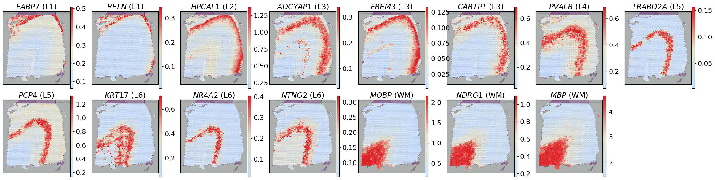
gene_list = ['FABP7', 'RELN', 'HPCAL1', 'ADCYAP1', 'FREM3', 'CARTPT', 'PVALB', 'TRABD2A',
             'PCP4', 'KRT17', 'NR4A2', 'NTNG2', 'MOBP', 'NDRG1', 'MBP']

gene_region = {
    'FABP7': 'L1', 'RELN': 'L1',
    'HPCAL1': 'L2',
    'ADCYAP1': 'L3', 'FREM3': 'L3', 'CARTPT': 'L3',
    'PVALB': 'L4',
    'TRABD2A': 'L5', 'PCP4': 'L5',
    'KRT17': 'L6', 'NR4A2': 'L6', 'NTNG2': 'L6',
    'MOBP': 'WM', 'NDRG1': 'WM', 'MBP': 'WM'
}

Gene expression visualization

[7]:

fig, axes = plt.subplots(2, 8, figsize=(24, 6))
axes = axes.flatten()

for i, gene in enumerate(gene_list):
    sc.pl.spatial(adata, layer='X_log', color=gene, cmap=gene_exp_palette, spot_size=150, ax=axes[i], show=False, img_key='hires',
                  vmax="p99", title=f"$\mathit{{{gene}}}$ ({gene_region[gene]})")
    axes[i].set_xlabel('')
    axes[i].set_ylabel('')
axes[-1].axis('off')

plt.tight_layout(pad=0.1)
plt.show()

[8]:

adata.X = adata.layers['STADIM'].copy()
sc.pp.log1p(adata)
adata.layers['STADIM_log'] = adata.X.copy()

fig, axes = plt.subplots(2, 8, figsize=(24, 6))
axes = axes.flatten()

for i, gene in enumerate(gene_list):
    sc.pl.spatial(adata, layer='STADIM_log', color=gene, cmap=gene_exp_palette, spot_size=150, ax=axes[i], show=False, img_key='hires',
                  vmax="p99", title=f"$\mathit{{{gene}}}$ ({gene_region[gene]})")
    axes[i].set_xlabel('')
    axes[i].set_ylabel('')
axes[-1].axis('off')

plt.tight_layout(pad=0.1)
plt.show()

WARNING: adata.X seems to be already log-transformed.

Evaluation metrics

[9]:

import os
import sys
from contextlib import redirect_stdout

results = []

for layer in ['X_norm', 'STADIM']:
    for gene, region in gene_region.items():
        expr = adata.layers[layer][:, adata.var_names.get_loc(gene)]
        expr = expr.toarray().flatten() if hasattr(expr, 'toarray') else np.array(expr).flatten()

        mask = adata.obs['Label'] == region
        target_val = expr[mask]
        bg_val = expr[~mask]

        with open(os.devnull, 'w') as fnull:
            with redirect_stdout(fnull):
                moran = stadim.calculate_new_morani(adata, [layer], {gene: region})

        results.append({
            'Method': layer,
            'Gene': gene,
            'Region': region,
            'Tau': stadim.calculate_tau_index(expr, adata.obs['Label']),
            'FC': stadim.calculate_fold_change(target_val, bg_val),
            'Cohens_D': stadim.calculate_cohens_d(target_val, bg_val),
            'Global_Moran': moran['Global_Moran'].values[0],
            'Background_Moran': moran['Background_Moran'].values[0],
            'newI': moran['newI'].values[0]
        })

df_res = pd.DataFrame(results)

[10]:

for layer in ['X_norm', 'STADIM']:
    print(f"\n=== Detailed Metrics for {layer} ===")
    layer_df = df_res[df_res['Method'] == layer]
    display(layer_df)

print("\n=== Final Summary (Averaged across all genes) ===")
summary = df_res.groupby('Method')[['Tau', 'FC', 'Cohens_D', 'Global_Moran', 'Background_Moran', 'newI']].mean()
display(summary.sort_values('newI', ascending=False))


=== Detailed Metrics for X_norm ===

	Method	Gene	Region	Tau	FC	Cohens_D	Global_Moran	Background_Moran	newI
0	X_norm	FABP7	L1	0.679730	3.176126	0.721098	0.089367	0.036577	0.526395
1	X_norm	RELN	L1	0.833288	7.612881	0.775069	0.109547	0.045728	0.531910
2	X_norm	HPCAL1	L2	0.699730	3.068554	1.360526	0.221055	0.135886	0.542585
3	X_norm	ADCYAP1	L3	0.561619	2.554207	0.353631	0.051692	0.009240	0.521226
4	X_norm	FREM3	L3	0.714852	3.003668	0.259095	0.047120	0.017907	0.514607
5	X_norm	CARTPT	L3	0.594013	3.195088	0.478894	0.124311	0.063235	0.530538
6	X_norm	PVALB	L4	0.596678	2.239379	0.565294	0.074833	0.057134	0.508850
7	X_norm	TRABD2A	L5	0.841705	7.867309	0.623517	0.071052	-0.006673	0.532189
8	X_norm	PCP4	L5	0.697033	3.536765	1.128401	0.253894	0.066206	0.593844
9	X_norm	KRT17	L6	0.758341	3.998996	0.796877	0.125162	0.045310	0.539926
10	X_norm	NR4A2	L6	0.719760	3.072878	0.330337	0.053665	0.049078	0.502294
11	X_norm	NTNG2	L6	0.455522	1.800602	0.241853	0.024883	0.000786	0.512048
12	X_norm	MOBP	WM	0.919297	11.077320	3.416460	0.710332	0.331313	0.689509
13	X_norm	NDRG1	WM	0.805246	4.729894	1.521295	0.268364	0.076004	0.596180
14	X_norm	MBP	WM	0.892194	8.341205	4.951767	0.909925	0.705406	0.602260


=== Detailed Metrics for STADIM ===

	Method	Gene	Region	Tau	FC	Cohens_D	Global_Moran	Background_Moran	newI
15	STADIM	FABP7	L1	0.581135	2.441201	3.132529	0.818420	0.757170	0.530625
16	STADIM	RELN	L1	0.717490	4.364239	2.716194	0.814868	0.769424	0.522722
17	STADIM	HPCAL1	L2	0.662147	2.710248	3.049344	0.857274	0.783988	0.536643
18	STADIM	ADCYAP1	L3	0.531298	2.405351	2.059148	0.814738	0.609914	0.602412
19	STADIM	FREM3	L3	0.667070	2.597443	1.546577	0.877676	0.704484	0.586596
20	STADIM	CARTPT	L3	0.568594	3.103972	2.004034	0.847647	0.755061	0.546293
21	STADIM	PVALB	L4	0.525031	1.971619	1.827773	0.845831	0.791697	0.527067
22	STADIM	TRABD2A	L5	0.802766	5.740999	2.960346	0.812605	0.380765	0.715920
23	STADIM	PCP4	L5	0.561332	2.447884	2.470404	0.835366	0.781112	0.527127
24	STADIM	KRT17	L6	0.741785	3.666232	2.546959	0.807889	0.594334	0.606777
25	STADIM	NR4A2	L6	0.738118	3.418727	1.538140	0.814291	0.634330	0.589981
26	STADIM	NTNG2	L6	0.434813	1.625638	1.125350	0.823101	0.784449	0.519326
27	STADIM	MOBP	WM	0.914177	10.399591	6.246632	0.957841	0.758200	0.599821
28	STADIM	NDRG1	WM	0.779575	4.257239	5.381348	0.958056	0.792414	0.582821
29	STADIM	MBP	WM	0.889637	7.987041	5.747448	0.952741	0.770116	0.591312


=== Final Summary (Averaged across all genes) ===

	Tau	FC	Cohens_D	Global_Moran	Background_Moran	newI
Method
STADIM	0.674331	3.942495	2.956815	0.855890	0.711164	0.572363
X_norm	0.717934	4.618325	1.168274	0.209013	0.108876	0.549624

Label specific markers

[11]:

def get_markers(adata, layer, n_top=100):
    key = f'rank_{layer}'
    sc.tl.rank_genes_groups(adata, 'Label', method='wilcoxon', layer=layer, key_added=key)
    df = sc.get.rank_genes_groups_df(adata, group=None, key=key)
    # Add rank and filter top N
    df['Rank'] = df.groupby('group').cumcount() + 1
    return df[df['Rank'] <= n_top][['names', 'group', 'Rank']].rename(columns={'names':'Gene', 'group':'Label'})

# 1. Get Top 100 markers for both layers
df_norm = get_markers(adata, 'X_log')
df_stadim = get_markers(adata, 'STADIM_log')

# 2. Merge to find common and unique pairs
merged = pd.merge(df_norm, df_stadim, on=['Gene', 'Label'], how='outer', suffixes=('_norm', '_stadim'), indicator=True)

common = merged[merged['_merge'] == 'both']
unique_norm = merged[merged['_merge'] == 'left_only']
unique_stadim = merged[merged['_merge'] == 'right_only']

# 3. Quick Stats Report
print(f"--- Marker Stats (Gene-Label Pairs) ---")
print(f"Common: {len(common)} | Unique Norm: {len(unique_norm)} | Unique STADIM: {len(unique_stadim)}")

# 4. Specificity Analysis: Multi-label genes (Noise Reduction)
multi_norm = df_norm.groupby('Gene')['Label'].nunique()
multi_stadim = df_stadim.groupby('Gene')['Label'].nunique()

# Genes that are multi-label in Norm but single-label (specific) in STADIM
denoised_genes = list(set(multi_norm[multi_norm > 1].index) & set(multi_stadim[multi_stadim == 1].index))

print(f"\n--- Specificity & Noise Reduction ---")
print(f"Multi-label genes in Norm: {sum(multi_norm > 1)}")
print(f"Multi-label genes in STADIM: {sum(multi_stadim > 1)}")
print(f"Denoised genes (Multi-label -> Single-label): {len(denoised_genes)}")

if denoised_genes:
    print(f"Denoised gene examples: {denoised_genes[:10]}")

--- Marker Stats (Gene-Label Pairs) ---
Common: 154 | Unique Norm: 546 | Unique STADIM: 546

--- Specificity & Noise Reduction ---
Multi-label genes in Norm: 162
Multi-label genes in STADIM: 0
Denoised genes (Multi-label -> Single-label): 34
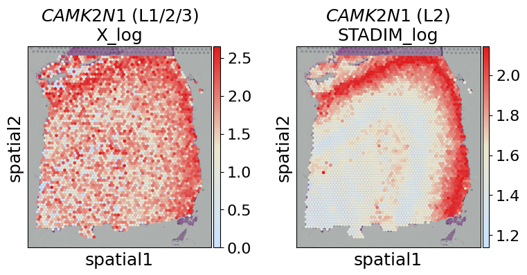
Denoised gene examples: ['CRYAB', 'DIRAS2', 'UBE2QL1', 'HS3ST2', 'NEFL', 'MAG', 'CAMK2N1', 'ENC1', 'CLDND1', 'ATP5F1B']

[12]:

merged[merged['Gene'] == 'CAMK2N1']

[12]:

	Gene	Label	Rank_norm	Rank_stadim	_merge
192	CAMK2N1	L1	31.0	NaN	left_only
193	CAMK2N1	L2	1.0	8.0	both
194	CAMK2N1	L3	28.0	NaN	left_only

[13]:

gene = 'CAMK2N1'
labels_gene = ['L1/2/3', 'L2']
layers = ['X_log', 'STADIM_log']

fig, axes = plt.subplots(1, 2, figsize=(8, 4))

for i, layer in enumerate(layers):
    sc.pl.spatial(adata, layer=layer, color=gene, cmap=gene_exp_palette, spot_size=150, vmax='p99',
                  ax=axes[i], show=False, title=f"$\mathit{{{gene}}}$ ({labels_gene[i]})\n{layer}")

plt.tight_layout()
plt.show()

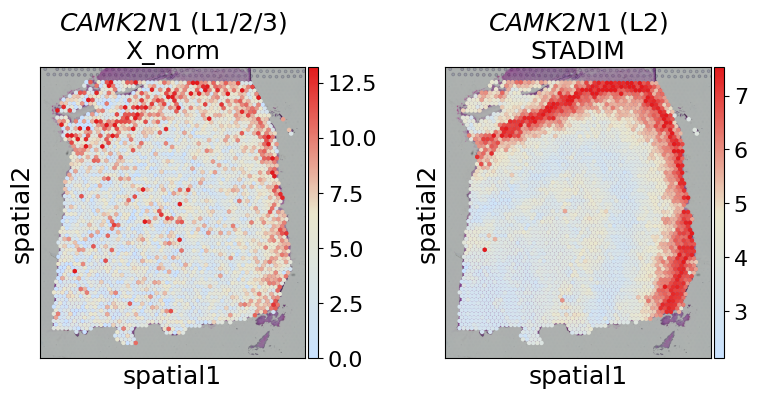
[14]:

gene = 'CAMK2N1'
labels_gene = ['L1/2/3', 'L2']
layers = ['X_norm', 'STADIM']

fig, axes = plt.subplots(1, 2, figsize=(8, 4))

for i, layer in enumerate(layers):
    sc.pl.spatial(adata, layer=layer, color=gene, cmap=gene_exp_palette, spot_size=150, vmax='p99',
                  ax=axes[i], show=False, title=f"$\mathit{{{gene}}}$ ({labels_gene[i]})\n{layer}")

plt.tight_layout()
plt.show()

[ ]:

[ ]: