Tutorial 2: Vertical denoising and integration on DLPFC multi slices from 10x Visium

In this tutorial, we evaluate the capability of STADIM in handling vertically adjacent slices. We use the human Dorsolateral Prefrontal Cortex (DLPFC) slice #151673-#151676 generated by 10x Visium platform as a representative example, which is annotated by Maynard et al. into white matter (WM) and cortical layers (L1-L6) based on marker genes and cellular structure.

We download the data via http://spatial.libd.org/spatialLIBD/.

Quick view data

[1]:

import scanpy as sc
import matplotlib.pyplot as plt
import os

sample_ids = ['151673', '151674', '151675', '151676']
data_dir = '/data2/xiaost/SODA/Data/DLPFC/'

fig, axes = plt.subplots(1, 4, figsize=(16, 4))

for i, s_id in enumerate(sample_ids):
    adata = sc.read_h5ad(os.path.join(data_dir, f'dlpfc_{s_id}.h5ad'))
    print(f'{s_id}')
    print(adata)

    sc.pl.spatial(adata, color='Label', ax=axes[i], show=False, title=f'Sample {s_id}')

    axes[i].set_xlabel('')
    axes[i].set_ylabel('')

plt.tight_layout()
plt.show()

151673
AnnData object with n_obs × n_vars = 3611 × 33538
    obs: 'in_tissue', 'array_row', 'array_col', 'sample', 'Label'
    var: 'gene_ids', 'feature_types', 'genome'
    uns: 'spatial'
    obsm: 'spatial'
151674
AnnData object with n_obs × n_vars = 3635 × 33538
    obs: 'in_tissue', 'array_row', 'array_col', 'sample', 'Label'
    var: 'gene_ids', 'feature_types', 'genome'
    uns: 'spatial'
    obsm: 'spatial'
151675
AnnData object with n_obs × n_vars = 3566 × 33538
    obs: 'in_tissue', 'array_row', 'array_col', 'sample', 'Label'
    var: 'gene_ids', 'feature_types', 'genome'
    uns: 'spatial'
    obsm: 'spatial'
151676
AnnData object with n_obs × n_vars = 3431 × 33538
    obs: 'in_tissue', 'array_row', 'array_col', 'sample', 'Label'
    var: 'gene_ids', 'feature_types', 'genome'
    uns: 'spatial'
    obsm: 'spatial'

Run STADIM

You can call the STADIM command directly in your terminal:

nohup stadim --input "./dlpfc_151673.h5ad" "./dlpfc_151674.h5ad" "./dlpfc_151675.h5ad" "./dlpfc_151676.h5ad" --save_dir ./dlpfc_donor1_test --device "cuda:0" --monitor --seed 2026 --min_genes 0 --min_cells 10 --knn_c 6 --knn_e 10 --mnn_n 25 > ./dlpfc_donor1_test.log 2>&1 &

and load the results into your Python environment for downstream analysis. The denoised expression matrix is conveniently stored within the layers attribute:

import anndata as ad

adata = ad.read_h5ad('/dlpfc_donor1_test/sdata.h5ad')

## The denoised gene expressionis is stored in adata.layers['STADIM']
print(adata)

or you can call STADIM within a Jupyter Notebook as follows:

[2]:

import stadim

adata = stadim.run_STADIM(['/data2/xiaost/SODA/Data/DLPFC/dlpfc_151673.h5ad', '/data2/xiaost/SODA/Data/DLPFC/dlpfc_151674.h5ad',
                          '/data2/xiaost/SODA/Data/DLPFC/dlpfc_151675.h5ad', '/data2/xiaost/SODA/Data/DLPFC/dlpfc_151676.h5ad'],
                          save_preprocessed_h5ad=None, save_dir=None,
                          sample_names=None, batch_key='sample', device='cuda:1', seed=2026,
                          min_genes=0, min_cells=10, nhvgs=2000, dim=50, knn_c=6, knn_e=10, mnn_n=25,
                          batch_size=256, triplets_update_ratio=0.8, hard_triplets_ratio=0.7,
                          epochs=100, lr=1e-3, loss_mode='nb', beta_trip=0.1,
                          encoder_layers=[512, 256, 64], decoder_layers=[1000])

Results will be stored in adata.layers['STADIM']

=== 1. Begin read_data!
Detected multi-slice data, total 4 slices
  Slice 1: Using user-defined column 'sample' as sample
  Slice 1: Keeping existing sample label 151673
  Slice 2: Using user-defined column 'sample' as sample
  Slice 2: Keeping existing sample label 151674
  Slice 3: Using user-defined column 'sample' as sample
  Slice 3: Keeping existing sample label 151675
  Slice 4: Using user-defined column 'sample' as sample
  Slice 4: Keeping existing sample label 151676

Merging data...

Raw Merged Data: 14243 spots × 33538 genes
Unified Filtering (min_genes=0, min_cells=10)...
  → After Filtering: 14243 spots × 19326 genes
  ✓ Complete: Samples included: ['151673', '151674', '151675', '151676']
  ✓ Complete: AnnData object with n_obs × n_vars = 14243 × 19326
    obs: 'in_tissue', 'array_row', 'array_col', 'sample', 'Label'
    var: 'gene_ids', 'feature_types', 'genome', 'n_cells'
    uns: 'spatial'
    obsm: 'spatial'
    layers: 'X_raw'

=== 2. Begin MY_preprocess!
== Selected 2000 HVGs across 4 slices

=== 3. Begin all_ap find neighbors!

=== 4. Begin pre_dataset!
{0: '151673', 1: '151674', 2: '151675', 3: '151676'}

Preparing triplet: 100%|██████████| 14243/14243 [00:02<00:00, 6902.20it/s]


=== 5. Begin IterableTripletDataset!
Initializing triplets...
IterableTripletDataset Initialized: 14243 anchors, batch_size=256

=== 6. Begin calculate_recommended_margin!
Calculating recommended margin (averaging over 5 runs)...

========================================
Margins from 5 runs: [15.0, 15.0, 15.0, 15.0, 15.0]
Final Recommended Margin: 15.0000

=== 7. Starting training...
Begin training: device=cuda:1

Training: 100%|██████████| 100/100 [05:23<00:00,  3.24s/it, recon=0.306, triplet=1.794, total=0.486]


=== 8. Generating denoised expression...
   Data size (2.75e+08) is within limits. Allocating memory for denoised data.

All processes finished! Total time: 6.62 mins.

[3]:

print(adata)

AnnData object with n_obs × n_vars = 14243 × 19326
    obs: 'in_tissue', 'array_row', 'array_col', 'sample', 'Label', 'n_genes_by_counts', 'log1p_n_genes_by_counts', 'total_counts', 'log1p_total_counts', 'size_factor'
    var: 'gene_ids', 'feature_types', 'genome', 'n_cells', 'n_cells_by_counts', 'mean_counts', 'log1p_mean_counts', 'pct_dropout_by_counts', 'total_counts', 'log1p_total_counts', 'highly_variable'
    uns: 'spatial', 'log1p', 'top_hvgs'
    obsm: 'spatial', 'S_scale', 'X_hvg_scale', 'X_pca', 'cell_names', 'STADIM'
    layers: 'X_raw', 'X_norm', 'X_log', 'STADIM', 'STADIM_withbatch'

Analysis

[4]:

import anndata as ad
import pandas as pd
import scanpy as sc
import numpy as np
import os
import warnings
warnings.filterwarnings('ignore')

import seaborn as sns
from matplotlib.colors import LinearSegmentedColormap
gene_exp_colors = sns.blend_palette(["#C9E2FF", "#eae6cc", '#e31a1c'], n_colors=100)
gene_exp_palette = LinearSegmentedColormap.from_list("gene_exp", gene_exp_colors)
import matplotlib.pyplot as plt
from matplotlib.lines import Line2D
import matplotlib.patches as mpatches
plt.rcParams.update({
    'font.size': 16,
    'axes.labelsize': 18,
    'axes.titlesize': 18,
    'xtick.labelsize': 16,
    'ytick.labelsize': 16,
    'legend.fontsize': 16,
})

styles = {
    'STADIM': {'color': '#d62728', 'marker': '*', 'ms': 10, 'lw': 2.5, 'zorder': 10},
    'X_norm': {'color': '#c7c7c7', 'marker': 'o', 'ms': 6, 'lw': 1.5, 'zorder': 5}
}

Gene expression visualization

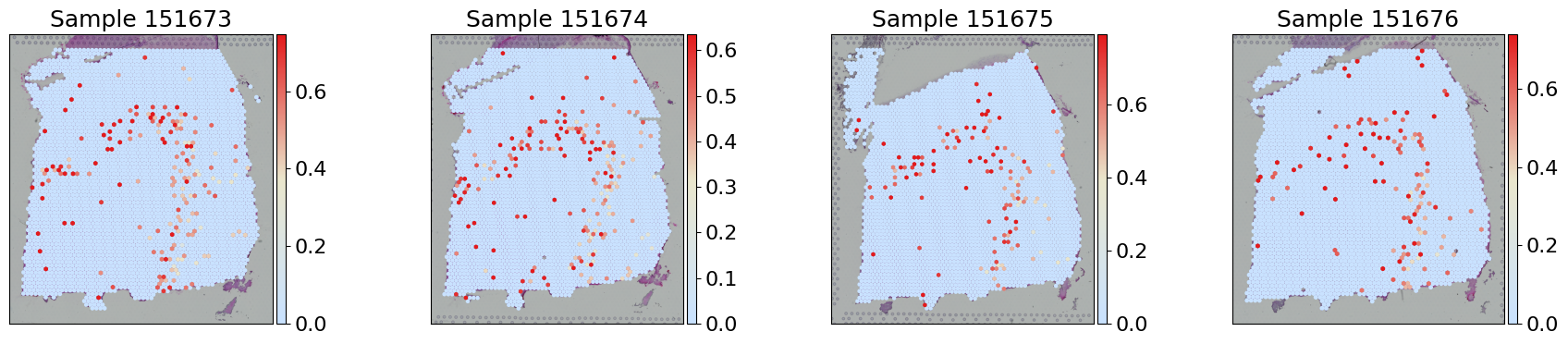
[5]:

fig, axes = plt.subplots(1, 4, figsize=(18, 4))
for i, s_id in enumerate(sample_ids):
    sc.pl.spatial(adata[adata.obs['sample'] == s_id], layer='X_log', color='TRABD2A', cmap=gene_exp_palette, spot_size=150,
                  library_id=s_id, ax=axes[i], title=f"Sample {s_id}",show=False, vmax='p99')
    axes[i].set_xlabel('')
    axes[i].set_ylabel('')

plt.tight_layout()
plt.show()

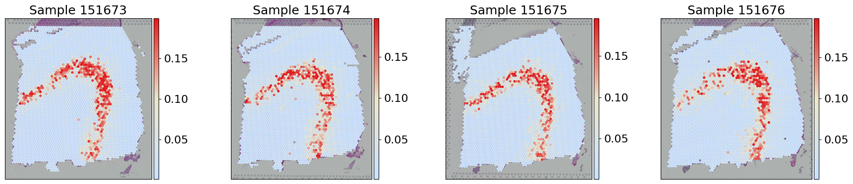
[6]:

adata.X = adata.layers['STADIM'].copy()
sc.pp.log1p(adata)
adata.layers['STADIM_log'] = adata.X.copy()

fig, axes = plt.subplots(1, 4, figsize=(18, 4))
for i, s_id in enumerate(sample_ids):
    sc.pl.spatial(adata[adata.obs['sample'] == s_id], layer='STADIM_log', color='TRABD2A', cmap=gene_exp_palette, spot_size=150,
                  library_id=s_id, ax=axes[i], title=f"Sample {s_id}",show=False, vmax='p99')
    axes[i].set_xlabel('')
    axes[i].set_ylabel('')

plt.tight_layout()
plt.show()

WARNING: adata.X seems to be already log-transformed.

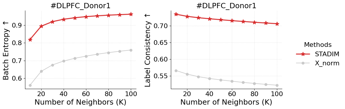
Batch Entropy

[7]:

%%time

res = stadim.calculate_batch_entropy(adata, test_layers=['X_norm', 'STADIM'], k_range=[10, 20, 30, 40, 50, 60, 70, 80, 90, 100],
                                     group_key='Label', donor_id='DLPFC_Donor1', batch_key='sample', n_hvg=2000)

batch_entropy = pd.DataFrame(res)

display(batch_entropy)

	Method	Donor_ID	K	Avg_Entropy	Avg_Region_Ratio
0	X_norm	DLPFC_Donor1	10	0.561502	0.566145
1	X_norm	DLPFC_Donor1	20	0.639298	0.555410
2	X_norm	DLPFC_Donor1	30	0.675469	0.547668
3	X_norm	DLPFC_Donor1	40	0.697315	0.542279
4	X_norm	DLPFC_Donor1	50	0.712926	0.537930
5	X_norm	DLPFC_Donor1	60	0.725089	0.534229
6	X_norm	DLPFC_Donor1	70	0.735988	0.530475
7	X_norm	DLPFC_Donor1	80	0.744872	0.527497
8	X_norm	DLPFC_Donor1	90	0.752677	0.524724
9	X_norm	DLPFC_Donor1	100	0.759480	0.522301
10	STADIM	DLPFC_Donor1	10	0.818788	0.734438
11	STADIM	DLPFC_Donor1	20	0.893744	0.728073
12	STADIM	DLPFC_Donor1	30	0.919236	0.723916
13	STADIM	DLPFC_Donor1	40	0.932822	0.720812
14	STADIM	DLPFC_Donor1	50	0.941357	0.717912
15	STADIM	DLPFC_Donor1	60	0.947545	0.715151
16	STADIM	DLPFC_Donor1	70	0.952164	0.712708
17	STADIM	DLPFC_Donor1	80	0.955841	0.710375
18	STADIM	DLPFC_Donor1	90	0.958784	0.708112
19	STADIM	DLPFC_Donor1	100	0.961284	0.706041

CPU times: user 1min 29s, sys: 3.89 s, total: 1min 33s
Wall time: 40.6 s

[8]:

metrics = ['Avg_Entropy', 'Avg_Region_Ratio']
y_labels = ['Batch Entropy \u2191', 'Label Consistency \u2191']

plot_data = batch_entropy.groupby(['Method', 'K'])[metrics].mean().reset_index()

fig, axes = plt.subplots(1, 2, figsize=(10, 4), sharex=True)

for i, metric in enumerate(metrics):
    ax = axes[i]
    for m in ['STADIM','X_norm']:
        data = plot_data[plot_data['Method'] == m].sort_values('K')
        if data.empty: continue

        ax.plot(data['K'], data[metric], label=m,
                color=styles[m]['color'], marker=styles[m]['marker'],
                markersize=styles[m]['ms'], linewidth=styles[m]['lw'],
                zorder=styles[m]['zorder'], alpha=0.9)

    ax.set_title(f"#DLPFC_Donor1")
    ax.set_xlabel('Number of Neighbors (K)')
    ax.set_ylabel(y_labels[i])
    ax.set_xticks([20, 40, 60, 80, 100])
    ax.grid(True, linestyle=':', alpha=0.5)
    sns.despine(ax=ax)

handles, labels = axes[0].get_legend_handles_labels()
fig.legend(handles, labels, loc='center left', bbox_to_anchor=(1.0, 0.5),
           title='Methods', frameon=False)

plt.tight_layout()
plt.show()

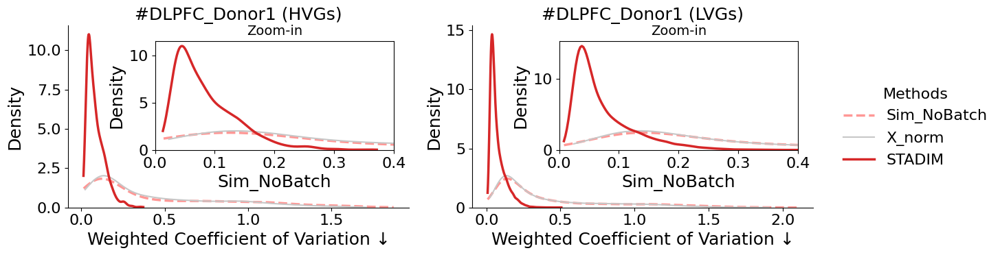
weighted Coefficient of Variation (wCV)

[9]:

benchmark_adata = stadim.create_shuffled_batches(adata, n_batches=5)
benchmark_adata.var = adata.var
print(f"\nbenchmark adata: {benchmark_adata}")


benchmark adata: AnnData object with n_obs × n_vars = 14243 × 19326
    obs: 'in_tissue', 'array_row', 'array_col', 'sample', 'Label', 'n_genes_by_counts', 'log1p_n_genes_by_counts', 'total_counts', 'log1p_total_counts', 'size_factor', 'sim_batch'
    var: 'gene_ids', 'feature_types', 'genome', 'n_cells', 'n_cells_by_counts', 'mean_counts', 'log1p_mean_counts', 'pct_dropout_by_counts', 'total_counts', 'log1p_total_counts', 'highly_variable'
    obsm: 'spatial', 'S_scale', 'X_hvg_scale', 'X_pca', 'STADIM'
    layers: 'X_raw', 'X_norm', 'X_log', 'STADIM', 'STADIM_withbatch', 'STADIM_log'

[10]:

%%time

wcv = {}
for gene_type in ["HVGs", "LVGs"]:
    print(f"\ngene_type: {gene_type}")

    # wCV before and after STADIM
    res_deno = stadim.calculate_cv(adata, batch_key='sample', label_key='Label', methods=['X_norm', 'STADIM'], gene_type=gene_type)

    # wCV of simulated benchmark no batch data, calculated with X_norm and shuffled labels
    res_bench = stadim.calculate_cv(benchmark_adata, batch_key='sim_batch', label_key='Label', methods=['X_norm'], gene_type=gene_type)
    res_bench = res_bench.rename(columns={'X_norm': 'Sim_NoBatch'})

    wcv[gene_type] = res_bench.join(res_deno, how='inner')

print(wcv["HVGs"].head())


gene_type: HVGs
--- Calculating CV on 2000 genes of type: HVGs ---
Methods successfully calculated: ['X_norm', 'STADIM']
--- Calculating CV on 2000 genes of type: HVGs ---
Methods successfully calculated: ['X_norm']

gene_type: LVGs
--- Calculating CV on 17326 genes of type: LVGs ---
Methods successfully calculated: ['X_norm', 'STADIM']
--- Calculating CV on 17326 genes of type: LVGs ---
Methods successfully calculated: ['X_norm']
            Sim_NoBatch    X_norm    STADIM
HES4           0.098084  0.125947  0.037362
VWA1           0.110024  0.116677  0.055306
AL645728.1     0.907844  0.635260  0.110994
FO704657.1     1.088555  0.903454  0.133141
AL109917.1     0.652083  0.713419  0.074418
CPU times: user 11.7 s, sys: 2.02 s, total: 13.7 s
Wall time: 13.7 s

[11]:

from mpl_toolkits.axes_grid1.inset_locator import inset_axes

methods = ['Sim_NoBatch', 'X_norm', 'STADIM']
colors = {'Sim_NoBatch': '#ff9896', 'X_norm': '#c7c7c7', 'STADIM': '#d62728'}
gene_types = ['HVGs', 'LVGs']


fig, axes = plt.subplots(1, 2, figsize=(12, 4))

for i, g_type in enumerate(gene_types):
    ax = axes[i]
    df = wcv[g_type]

    ax_ins = inset_axes(ax, width="70%", height="60%", loc=1, borderpad=1)

    for m in methods:
        if m not in df.columns: continue

        style = {
            'label': m, 'color': colors.get(m, '#333333'), 'fill': False,
            'linewidth': 2.5 if m != 'X_norm' else 1.5,
            'linestyle': '--' if m == 'Sim_NoBatch' else '-',
            'zorder': 10 if m == 'STADIM' else 5,
            'cut': 0
        }

        sns.kdeplot(df[m].dropna(), ax=ax, **style)
        sns.kdeplot(df[m].dropna(), ax=ax_ins, **style)

    ax.set_title(f"#DLPFC_Donor1 ({g_type})")
    ax.set_xlabel("Weighted Coefficient of Variation \u2193")
    ax_ins.set_xlim(0, 0.4)
    ax_ins.set_title("Zoom-in", fontsize=14)
    sns.despine(ax=ax)

handles, labels = axes[0].get_legend_handles_labels()
fig.legend(handles, labels, loc='center left', bbox_to_anchor=(1.0, 0.5),
           title='Methods', frameon=False)

plt.tight_layout()
plt.show()

Latent representation Umap

[12]:

%%time

sc.pp.neighbors(adata, use_rep='STADIM', key_added=f'neighbors_STADIM')
sc.tl.umap(adata, neighbors_key=f'neighbors_STADIM')
adata.obsm['X_umap_STADIM'] = adata.obsm['X_umap'].copy()
print(adata)

AnnData object with n_obs × n_vars = 14243 × 19326
    obs: 'in_tissue', 'array_row', 'array_col', 'sample', 'Label', 'n_genes_by_counts', 'log1p_n_genes_by_counts', 'total_counts', 'log1p_total_counts', 'size_factor'
    var: 'gene_ids', 'feature_types', 'genome', 'n_cells', 'n_cells_by_counts', 'mean_counts', 'log1p_mean_counts', 'pct_dropout_by_counts', 'total_counts', 'log1p_total_counts', 'highly_variable'
    uns: 'spatial', 'log1p', 'top_hvgs', 'neighbors_STADIM', 'umap'
    obsm: 'spatial', 'S_scale', 'X_hvg_scale', 'X_pca', 'STADIM', 'X_umap', 'X_umap_STADIM'
    layers: 'X_raw', 'X_norm', 'X_log', 'STADIM', 'STADIM_withbatch', 'STADIM_log'
    obsp: 'neighbors_STADIM_distances', 'neighbors_STADIM_connectivities'
CPU times: user 4min 28s, sys: 225 ms, total: 4min 28s
Wall time: 1min 3s

[13]:

fig, axes = plt.subplots(1, 2, figsize=(8, 3))

sc.pl.embedding(adata, basis='X_umap_STADIM', color='Label', ax=axes[0], show=False, legend_loc='on data', legend_fontweight='normal',
                title='STADIM (Label)', frameon=False, s=15)

sc.pl.embedding(adata[np.random.permutation(adata.n_obs)], basis='X_umap_STADIM', color='sample', ax=axes[1], show=False,
                title='STADIM (Sample)', frameon=False, s=15)

plt.tight_layout()
plt.show()

[ ]:

[ ]: